2006-05-01
Abstract
Oren Drori and Nicky Pappo introduce their new model for calculating malware penetration probability during an outbreak.
Copyright © 2006 Virus Bulletin
This article presents a new model for calculating malware penetration probability during an outbreak. We suggest that the Malware Penetration Index (MPI) model should be adopted and developed further to become a standard calculation for the probability of malware penetration.
In this article we describe the motivation behind this initiative, elaborate on the theoretical model for the MPI and the methods for MPI estimation and calculation. Finally, we outline some possible real-life applications of the MPI model.
Today, the majority of malware is weighted and described differently by different anti-virus vendors, IT forums and analysts; even the media gives different definitions or threat levels for the same attack. In most cases, the severity of an attack is determined by its incurred damage. As a result, the most prevalent/widespread malware gains public exposure (often resulting in a global panic), while less widespread malware may barely be acknowledged.
Unfortunately this gives a value to only one aspect of the attack. Given that an increasing number of high-risk threats are being propagated as collections of multiple low-risk malware, it is essential that a complementary metric is defined to help measure the potential risks faced by organizations.
The MPI was developed to empower the community of IT professionals worldwide. It aims to provide a reliable, unified and vendor-independent forecasting procedure that can determine how well an organization is protected against new malware.
The MPI is a metric of a virus outbreak. Its aim is to indicate the chances of a virus-carrying email penetrating a user's mailbox.
The MPI paradigm has several desirable attributes:
Methodological and mathematically well-defined: its methodology makes it easy for users to understand what can and cannot be determined from this measure. The model's transparency invites open debate and scientific criticism.
Quantified: the MPI provides a comparison scale for virus outbreaks – for example, virus A has a larger or smaller MPI value than virus B.
Vendor-independent: in theory, any two people should be able to calculate the MPI for a given virus and reach the same answer (excluding errors in measurement). The MPI model is objective, and not based on the decisions of individual vendors or service providers.
MPI is the probability that a random virus-carrying message received during an attack will penetrate an organization’s anti-virus defence and arrive in an end user's mailbox.
The MPI value is affected both by the distribution of the virus and by the level of defences that have been deployed against it (at least in the target population).
| Driving factor | Impact on MPI value | |
|---|---|---|
| Attack parameters | Intensity | Increases |
| Shape of distribution | Right tail distribution curve (most volume distributed early): increases | |
| Left tail distribution curve (most volume distributed late): decreases | ||
| Attack speed | Increases | |
| AV parameters | Responsiveness of AVs | Increases |
| Number of effective AVs | Increases | |
| Identity of effective AVs | Large market share: increases | |
| Smaller vendors: decreases |
Table 1. MPI driving factors.
The following semantics are used in the MPI model:
Intensity level = the virus proportion (%) of the total traffic, at time t.
Miss rate = the proportion of the population that is unprotected at time t.
Penetration rate = at time t, the probability of a (random) received message being a successfully penetrating virus i.e. satisfies two conditions: the message carries a virus, and the user is unprotected (at time t).
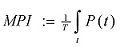
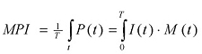
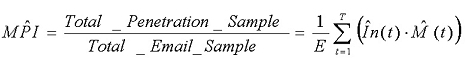
Malware Penetration Index:
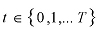
Attack length i.e.
Number of available anti-virus engines i.e.

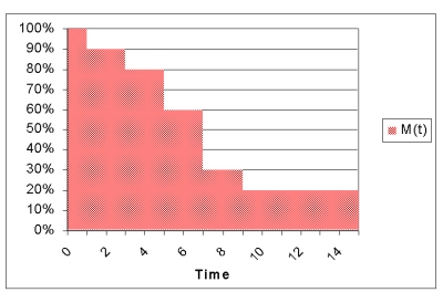
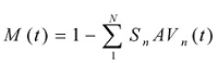
The miss rate function, M(t), is the percentage of users that are unprotected.
When M(t) is plotted against time, we typically see a descending step shape (see Figure 1). This is because every time a new anti-virus signature is released, an entire population of users change their status from unprotected to protected.
The requirements for calculating M(t) include determining which anti-virus products provide protection against the virus at time t, and determining the relative market share(s) of the various anti-virus product(s).
Additional definitions:
 defines whether anti-virus engine n provides protection against the virus. The answer is time-dependent, and it can be assigned a value of zero (0) if the answer is no, or a value of one (1), if the answer is yes.
Sn is the market share of anti-virus engine n. This means the proportion of users across the world that use this specific anti-virus product.
Aggregating the miss rate across anti-virus engines yields the following calculation:
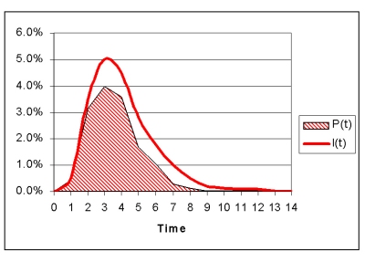
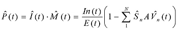
Penetration rate at time t is the product of the miss rate and the intensity (the prevalence of the virus, in percentage points):
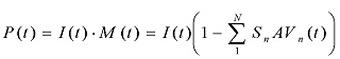
An example of a typical penetration rate graph is shown in Figure 2. It is calculated by multiplying the miss rate M(t) and the intensity I(t).
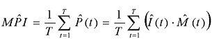
The MPI is the probability that a single (random) message that was sent at any time during an attack will become a penetrating message. In order to calculate this probability, it is necessary to calculate the proportion of the messages that were sent during that attack that answer the penetration criteria:
Note: Division by T is required in order to normalize the index to (0,1) range (between 0 and 100%).
In order to estimate the MPI for a message, we need to do the following:
Approximate the AVn(t) – mapping which anti-virus engine was added and when.
Approximate the Sn – market share of the various anti-virus engines.
Calculate the approximated value for M(t) – miss rate at time t.
Estimate I(t) – distribution intensity through the attack.
Estimate the penetration rate (at time t) and MPI.
In order to approximate AVn(t) we require a lab that has access to the various anti-virus products that are currently available, and which is updated throughout the attack. An independent lab such as AV-test.org could be used for this task. Such a lab might not cover every anti-virus engine on the market, but would provide a good approximation.
We also require a methodology for testing the different anti-virus engines at time t and repeatedly until the attack is over. Commtouch has built an automated mechanism that performs this action and then repeats it, once it is triggered.
More importantly, the above test must be performed from the beginning of the attack. A good zero-hour detection mechanism (signature- and update-independent) must be used for the trigger.
Approximating the market share of the anti-virus engines can be difficult for a number of reasons. First, the definition of market share is not trivial because analysts use different definitions of the market. In the MPI context the definition should be conclusive and include software solutions as well as hardware solutions, desktop as well as gateway products, consumer as well as business solutions.
Second, some users do not buy a pure anti-virus product, but rather a security package that includes virus protection. Anti-virus market researchers usually disregard these users.
Finally, market share is usually judged by revenue, while the MPI measurement requires market share to be determined by number of units.
In the example we have used, the approximate market share value (Sn) has been calculated by using a revenue breakdown as published by IDC.
Notes and reservations:
This approximation will serve reasonably on a global level (MPI as a proportion of infected and penetrating emails out of world traffic), but should be modified if one wishes to calculate the MPI for a particular market segment, such as business users or consumers etc.
Inclusion of integrated products in IDC's report is very partial, which creates a certain bias.
Using the approximated AVn(t) and Sn, you should have the required information to calculate the M(t) variable. To do this, consider a four-hour attack, approximated market share data and protection indications across the attack timeline (provided by a lab e.g. AV-test.org). Figure 3 illustrates the calculation of miss rate at various times – M(t).
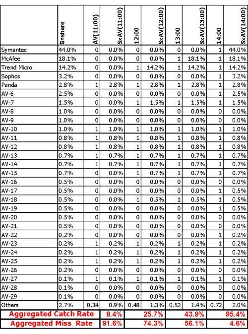
Figure 3. Example approximation of market share, Sn, and miss rate, M(t). Notes: 1. Market shares of the top five vendors are based on ‘Worldwide Antivirus 2005–2009 Forecast and Analysis’, IDC 2006. 2. Market shares of other vendors are approximated, using cross-match between a few sources – hence, the vendors are not specified by name. 3. ‘Others’ represent AV products for which we had no detection data: The total market share of these products is under 3%. Ignoring these products is equivalent to assigning them with ‘zero’ value. In order to avoid such bias, we are assuming their AV value is the average value in the industry at that time.
Intensity must be estimated based on a sample group. If the sample group is large enough and unbiased, the estimated I(t) will be an unbiased estimator.
The larger the sample group, the more accurate the estimation will be, and the more widespread the sample is (geographically, by email market segments etc.), the smaller the chances for bias will be. Î(t), the estimated intensity, is calculated as:
 where In(t) is the number of infected messages in the sample (between time t and t–1); E(t) is the size of the email sample between time t and t–1 and E is the size of the total email sample, through the attack, that is:

 , the estimated penetration rate at time t, is calculated as follows:
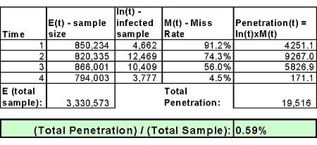
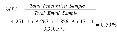
Alternatively, we can use the following simplified calculation, and more importantly, the process of data collection:
The two calculations are identical provided that email traffic is distributed evenly through the attack, i.e. E(t) = E(t´) for any t, t´. This assumption is more plausible when short attacks are considered, than for longer, slower attacks. Figure 4 shows an example for estimation.
As:
The above information is sufficient to draw the following conclusions:
MPI = (by definition) the proportion of emails that were both infected and reached unprotected user. For example: '1 of every XX emails through this attack has infected a user'.
MPI = the probability of a (randomly selected) individual message, sent sometime in the attack, being a successfully penetrating virus.
For attacks A and B that lasted for similar periods of time: if virus attack A has a higher MPI value than virus attack B, the chances of getting hit by virus A are greater than virus B.
Alternatively, it is possible to multiply the attack's MPI by the attack length (hours) and compare between any two attacks.
The MPI can be used for estimating the probability of a random user receiving the virus, however several steps and assumptions are required:
The probability must take into account the attack duration, and the number of emails received through that period of time.
Per received message (through the attack timeframe) the probability of getting hit is the MPI and the probability of not getting hit is 1 – MPI. [This is an approximation, ignoring the time of the specific message. If we consider the receiving time, t, of each message, the probabilities are P(t) and 1 – P(t).]
If we assume independence between the different emails received by the same user, and the approximation above (i.e. using MPI as hit probability for each message), the probability of not getting hit by any message = the probability of not getting hit by the first, and not getting hit by the second, etc. That is, Pr(safe) = (1 – MPI)X, where X is the number of messages received throughout the attack. The probability of getting hit through the attack, would then be: Pr(hit) = 1 – (1 – MPI)X.
For example, consider the following situation: a corporate user receives two emails per hour on a week day (about 50 a day). The attack takes place on a Tuesday and lasts 10 hours. The calculated MPI was 0.5%
Based on the above parameters, the total number of emails received was 20, and the probability of getting hit would be:
Pr(hit) = 1 – (1 – 0.005)20 = 1 – 0.905 » 9.5%
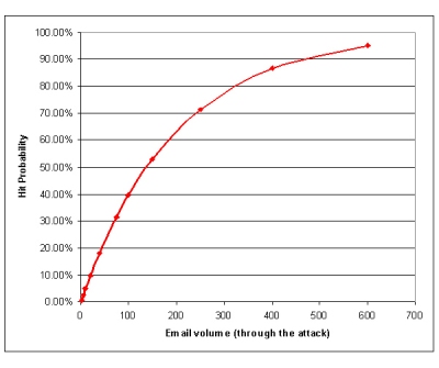
The hit probability responds dramatically to the first few emails received, while it is much less sensitive to whether 100 or 1000 messages have passed through:
| aMPI | 0.5% | |||
| Total emails | 1 | 10 | 100 | 400 |
| Hit probability | 0.50% | 4.89% | 39.42% | 86.53% |
Table 2. Hit probability sensitivity to email volume
However, even small changes in the MPI have a dramatic effect on the hit probability. In the example shown in Table 3, a rise in the MPI from 0.1% to 0.5% increases the hit probability from one in ten users to almost 40%. If the MPI reaches the 3% level, the chances of getting hit are a near certainty:
The MPI, a new virus metric, is a vendor-independent and quantified measure, focused on the penetration probability measure of a virus (or other malware) rather than on commonly examined aspects such as severity of damage. We have seen that, while there are challenges, it is possible to estimate the MPI in real life, providing one is willing to tolerate certain approximations.
The relevant application of the MPI for the IT community is the derivation of the hit probability, per user (based on the user's email usage pattern).
We welcome further discussion – please send us your feedback and related ideas to: <[email protected]>.