2012-10-10
Abstract
In the first two parts of this tutorial series Aleksander Czarnowski has demonstrated some useful manual tricks that are helpful in unpacking x64 binaries. In this third article he describes one more manual unpacking approach then moves on to some scripting examples.
Copyright © 2012 Virus Bulletin
In previous parts of this tutorial series [1], [2] I’ve given the same basic background on the difference between Windows on 32- and 64-bit platforms and demonstrated some useful tricks that are helpful in unpacking x64 binaries. However, each of the methods discussed so far has had one drawback: since they are manual they do not scale well. In the real world, binary instrumentation and automation of the unpacking process is a must.
In this article I’ll describe one more manual unpacking approach which is quite different from the methods already discussed, and then I’ll move on to some scripting examples. Each solution presented in this article requires only one tool: IDA.
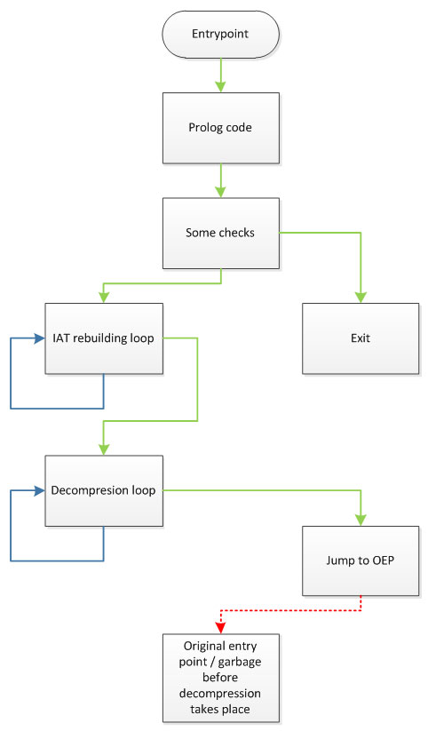
IDA has a couple of extremely useful graph features. Graph data can be extracted for additional analysis or manipulation through SDK or IDAPython interfaces, for example. We can use graph properties as an aid in the process of searching for the Original Entry Point (OEP). Even without reverting to the material presented in [1] and [2], we can imagine that somewhere within the decompression/IAT rebuild/obfuscation code must probably exist a single exit point which transfers execution flow to the original entry point. Now imagine such a flowchart graph – it should be similar to the one presented in Figure 1.
This clearly shows that one of the bottom graph nodes should be transferring execution to the original entry point. Since this is an interesting theory, let’s check it in practice using our test file from [1]:
Load the test file into 64-bit IDA.
Accept all warnings regarding IAT table corruption and allow IDA to load the file and create the assumed IAT automatically.
Select the ‘Local Bochs Debugger’ option from the ‘Choose debugger’ menu (don’t forget to configure the Bochs plug-in to handle 64-bit PE files).
Select the ‘Stop on entry point’ option in the ‘Debugger option’ menu.
Run the target process (F9 – start process).
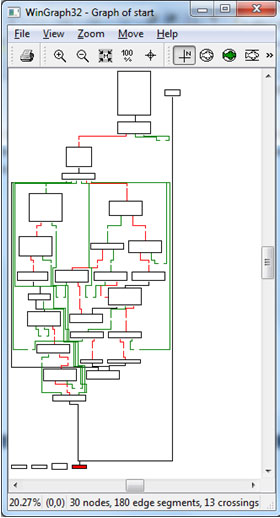
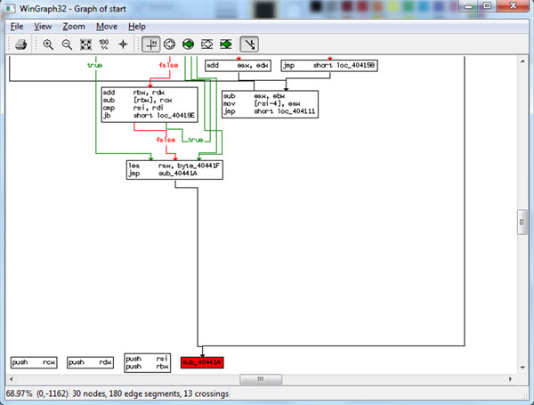
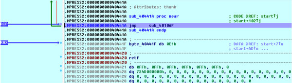
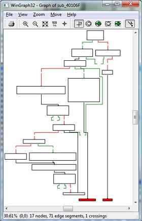
IDA debugger should stop at the address .MPRESS2:00000000004040C2 (in short form 0x04040C2) where the PUSH RDI instruction is located. Now, from the ‘Views’->‘Graphs’ menu, select the ‘Flowchart’ option (F12). A picture similar to Figure 2 should be displayed. Now zoom in (Figure 3) to reveal the bottom nodes and sub_40441A. Jump to this subroutine (press ‘g’ and enter ‘sub_40441A’ as the address – IDA will resolve it correctly) and place a breakpoint on it. Figure 4 shows the disassembly of this procedure. Note that this procedure is just a single JMP instruction and higher addresses (the lower part of the disassembly listing) are occupied by garbage bytes. Those bytes could be the compressed image or some other data (including real garbage) but they are definitely not a valid code area. Further analysis reveals that this is not the original entry point. So far it seems our theory isn’t valid. But before we come to any conclusion let’s get back to our imaginary flowchart in Figure 1. The bottom (exit) nodes from the entry point may lead to further parts of decompression routines. Therefore our theory could still be valid, and to prove it we need to inspect further functions which are bottom nodes on our graph.
Now let’s follow the jump using the ‘Step into’ option (F7). We land at the .MPRESS1:000000000040106F function (sub_40106F) and IDA stack analysis fails here. Once again, use the ‘Flowchart’ option (F12) – the result is shown in Figure 5.
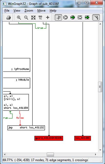
Scroll the graph to the bottom and zoom into the two red nodes (Figure 6).
Inspection of loc_40108C reveals a strange near call and some garbage code after the call instruction. If you fix the call address, changing it from loc_401AC+1 to loc_401AD, the proper disassembly of the called function will look like this:
.MPRESS1:00000000004010AD loc_4010AD:        ; CODE XREF: .MPRESS1:000000000040109Fp
.MPRESS1:00000000004010AD pop     rcx
.MPRESS1:00000000004010AE call    GetModuleHandleA
.MPRESS1:00000000004010B3 or      rax, rax
.MPRESS1:00000000004010B6 jz      short loc_401103
.MPRESS1:00000000004010B8 call    near ptr loc_4010C9+3
.MPRESS1:00000000004010BD push    rsi
.MPRESS1:00000000004010BE imul    esi, [rdx+74h], 506C6175h
.MPRESS1:00000000004010C5 jb      short near ptr loc_401135+1
.MPRESS1:00000000004010C7 jz      short near ptr loc_40112D+1
.MPRESS1:00000000004010C9
.MPRESS1:00000000004010C9 loc_4010C9:        ; CODE XREF: .MPRESS1:00000000004010B8p
.MPRESS1:00000000004010C9 movzx   rsi, dword ptr [rax+rax+5Ah]
.MPRESS1:00000000004010CD push    rax
.MPRESS1:00000000004010CE pop     rcx
.MPRESS1:00000000004010CF call    GetProcAddress
The calls to GetModuleHandleA and GetProcAddress make this function’s purpose quite obvious – although note that this is not the IAT rebuilding loop yet. Again, this is not our exit to the original entry point.
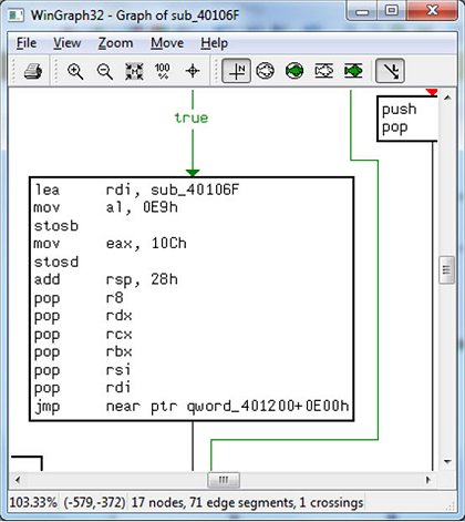
Let us examine the second red node – if you trace its caller (Figure 7) you will find that it is the short procedure which restores general registers from the stack and that it ends with a strange jump. Put a breakpoint at the jump and execute the process again (F9). Further analysis will reveal that this is in fact a jump to the original entry point. This proves that our theory was correct. What is more important is that the demonstrated method is generic and can be applied not only to different decompression/obfuscation schemes but to other executable file formats, processors and system platforms as well.
Please note that the assumptions made here are not entirely valid in the case of ‘virtualizing’ original code before compression/further obfuscation. In such cases the original entry point does not give us much information since the original native code is in the form of bytecode for the virtual (imaginary) processor. Decompilation in order to return to native code is beyond the scope of this tutorial.
A new feature called ‘trace replayer’ was introduced in IDA 6.3. This is a form of specialized debugger that allows the execution flow to be recorded. This feature can be used for unpacking as well. Again, we need to make some assumptions to start. Our first assumption will be that every user-land PE process ends with the ExitProcess() function. If the decompression/deobfuscation process works correctly, when reaching the original entry point the process should not crash or call ExitProcess. The ExitProcess call should be made from the original code when the main function exits. Note that when we refer to the main function we do not consider the C/C++ main() function.
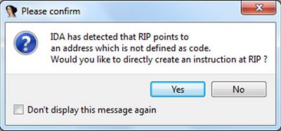
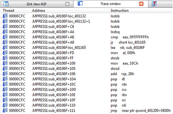
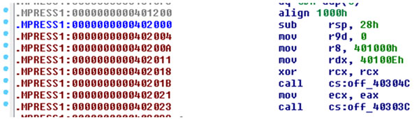
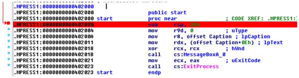
To demonstrate the use of trace replayer let’s load our sample file into IDA again (remember this will not work in versions older than 6.3) and again select ‘Local Bochs debugger’, enabling a break at the entry point option. When the breakpoint is hit, enter a breakpoint at the kernel32_ExitProcess function and select from the ‘Debugger’ menu the ‘Tracing’->‘Instruction tracing’ option. Now run the process again (F9) and wait… it might take a longer time since neither instruction tracing (which, internally, is automatic single stepping) nor Bochs emulation are speedy daemons. When the ExitProcess breakpoint is finally hit, select the ‘Trace window’ option from the ‘Debugger’->‘Tracing’ menu. Jump to the end of the trace listing and move upwards. Finally you will find JMP NEAR PTR QWORD_401200+0E00h – this is the jump to the original entry point. If you click on the next address (.MPRESS1:qword_401200+E00) at the trace window, IDA will ask you if this RIP location should be defined as code (see Figure 8): agree. Our trace should look like that shown in Figure 9. If you click on the next location after JMP you will see our main code disassembly starting from the original entry point:
1:0000000000401200 align 1000h
.MPRESS1:0000000000402000 sub      rsp, 28h
.MPRESS1:0000000000402004 mov      r9d, 0
.MPRESS1:000000000040200A mov      r8, 401000h
.MPRESS1:0000000000402011 mov      rdx, 40100Eh
.MPRESS1:0000000000402018 xor      rcx, rcx
.MPRESS1:000000000040201B call     cs:off_40304C
.MPRESS1:0000000000402021 mov      ecx, eax
.MPRESS1:0000000000402023 call     cs:off_40303C
Just like the previous method, the trace replayer can be used in the unpacking of files other than x64 PE files. It also works with other debuggers so it is possible to use it in conjunction with a remote debugger, for example. Single stepping is already time consuming, and Bochs adds an additional delay since it is an emulator. In the case of files that are larger than our example, tracing can take more time than is acceptable. In such cases switching from Bochs to a real operating system can help.
There are more features to the trace replayer than those shown here, including the colouring of executed areas of code etc.
While trace replayer adds some automation to our unpacking process it still requires some manual interaction. This is where IDA IDC and IDAPython functionality comes to the rescue. Since IDA also supports plug-in architecture you might consider this option including developing plug-ins using C/C++. On the other hand, IDC and IDAPython allow more rapid development and are available in a more dynamic way. Additionally, IDA already allows IDAPython and IDC scripts to be loader and processor modules.
As with previous examples, we need to start with some assumptions regarding the original entry point. One assumption that we can make is that since decompression/deobfuscation code is being added to the already linked PE file, it can attach itself as a last section. This should lead to a situation where the instruction that jumps to the original entry point has a higher address than its target. Since there are many different ways to transfer control for generic solutions we can’t rely on JMP instruction opcodes for detecting the jump to the original entry point. However, we can try to assume that if the RIP register points below our executable module entry point, we might have found the original entry point address. Now let’s implement this idea in IDAPython:
start_addr = BeginEA()
RunTo(start_addr)
GetDebuggerEvent(WFNE_SUSP, -1)
EnableTracing(TRACE_STEP, 1)
code = GetDebuggerEvent(WFNE_ANY | WFNE_CONT, -1)
if code:
    while code > 0:
        if GetEventEa() < start_addr:
            break
        code = GetDebuggerEvent(WFNE_ANY | WFNE_CONT,-1)
    PauseProcess()
    GetDebuggerEvent(WFNE_SUSP, -1)
    EnableTracing(TRACE_STEP, 0)
    MakeCode(GetEventEa())
    TakeMemorySnapshot(1)

Listing 1: Generic, simple OEP finder based on [3].
The following is a brief description of the functions used:
BeginEA() returns the address of the entry point identified by IDA during automatic analysis or the entry point address entered manually by the user.
RunTo() runs the process under selected debugger control and breaks at the specified address.
GetDebuggerEvent() takes two arguments: WFNE_* constants and timeout value. If the timeout value is set to -1 it means infinity, while any other number defines the number of seconds to wait. It is crucial to understand that GetDebuggerEvent() must be called after every execution break. The list of WFNE_* constants can be found in the IDA help file. The flags we are using: WFNE_ANY | WFNE_CONT mean that any first debugging event will be returned to our script (even if it does not suspend the debugged process execution) and continuation should be resumed from the suspended state. The WFNE_SUSP means that the script should wait until the process is suspended.
PauseProcess() suspends the running process under debugger control.
EnableTracing() enables debugger step tracing according to the trace_level value which is the first argument. TRACE_STEP (the lowest level trace – records all instructions), TRACE_INSN (records instruction trace) and TRACE_FUNC (records calls and rets) are possible options. The second argument, called enable, can have one of two values: 0 = turn off; 1 = turn on.
MakeCode() instructs IDA to treat the byte stream as code at the location pointed to by the argument.
TakeMemorySnapshot() takes a memory snapshot of the debugged process, meaning that debugger disassembly is transferred into the IDA database. This enables the results of dynamic analysis to be stored in a static disassembly produced by IDA at start-up.
Unfortunately, the example script will fail on our sample file since the original code is above and not below the decompression loop. However, it contains almost all the pieces necessary to build a working solution (remember always learn from your failures).
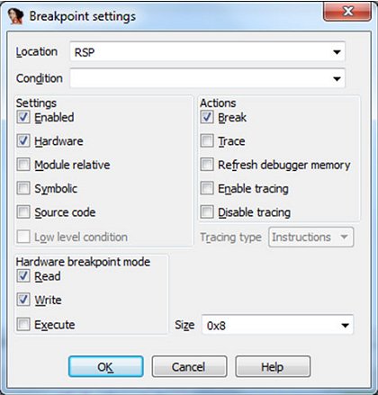
If you go back to the WinDbg discussion [2] you will find a method based on setting hardware breakpoints on the stack pointer at the beginning of the decompression code, which happens to be the entry point in our case. The same approach can be used with IDA, and thanks to the IDC/IDAPython interfaces it can quite easily be automated. First – as an exercise – try to unpack our target file manually. The local Bochs debugger is perfect for the job. Launch it and enable a break at the entry point option. Next, step over one instruction and set up a hardware breakpoint just as shown in Figure 10.
Now run the process again (F9) and wait until the breakpoint is hit. The result should be the same as that acquired with WinDbg. Now we can write a script that simulates our manual actions.
entry_addr = BeginEA()

entry_seg = SegName(entry_addr)

print ‘[*] Entry point: %s:%X’ % (entry_seg,entry_addr)

RunTo(entry_addr)

GetDebuggerEvent(WFNE_SUSP, -1) #page 533

StepInto()

GetDebuggerEvent(WFNE_SUSP, -1)

_rsp = cpu.Rsp

AddBptEx(_rsp, 0x8, BPT_RDWR)

code = GetDebuggerEvent(WFNE_ANY | WFNE_CONT, -1)

GetDebuggerEvent(WFNE_SUSP, -1)

curr_addr = ScreenEA()

bOk = False
i = 0

while i < 4:
     StepInto()
     if curr_addr > ScreenEA() + 0x100:
           bOk = True
           break
     if curr_addr < ScreenEA() - 0x100:
           bOk = True
           break
     GetDebuggerEvent(WFNE_SUSP, -1)
     i+=1

if bOk:
    _addr = ScreenEA()
    _seg = SegName(_addr)
    print ‘[*] Entry point found: %s,%X’ % (_seg, _addr)
    TakeMemorySnapshot(1)
else:
    print ‘[*] Failed to find entry point’

Listing 2: IDAPython script – stack hardware breakpoint generic unpacker.
Looking at listing 2, most of the functions used have been discussed already. Here are a couple of new ones:
SegName() returns the segment name of an address – as discussed in the first part of this tutorial segments are not PE sections but can mimic them in a way. From IDA’s perspective a segment is a logical unit used to identify and separate different areas of a loaded file.
StepInto() executes one step in the debugger.
cpu.Rsp gives us access to the RSP register value.
AddBptEx() allows us to add hardware breakpoints.
ScreenEA() returns the linear address of the cursor – in our case the cursor is being set at the correct place by the script.
After the hardware breakpoint is hit we take four StepOver() function calls until the current address is lower or greater than the current one by 0x100. This value is an arbitrary guess based on the idea that inside the decompression loop you can have RIP changing instructions like conditional jumps or calls to subroutines but none of them should be located far away from the caller. A bigger change of RIP value suggests the presence of the original entry point. Obviously, the 0x100 value can be changed. If the RIP value hasn’t changed during four iterations then scripts decide it failed in finding the OEP. Obviously the iteration number in the while loop can be changed too.
Note that after every StepInto() function call there is a companion GetDebuggerEvent call. Otherwise neither the StepInto() nor the StepOver() function would work properly. This means that the following code is invalid:
StepOver()
StepOver()
StepOver()
While this code will work correctly:
StepOver()
GetDebuggerEvent([...])
StepOver()
GetDebuggerEvent([...])
StepOver()
GetDebuggerEvent([...])
Since version 4.9, IDA has come with a Universal PE Unpacker plug-in, but it can’t handle our test file. Newer plug-ins (which can be used from IDA version 6.2 onwards with Bochs and 64-bit PEs) aid the unpacking process for PE files in uunp: Universal Unpacker Manual Reconstruct. This plug-in has already been mentioned in [1]. Now, when several different approaches to finding the OEP have been discussed, we can feed uunp with all the required data. The one thing uunp is helpful with and that we haven’t really discussed yet is the Import Address Table (IAT) rebuilding process. If the original IAT is large this could be quite a tedious process, hence automating it with a plug-in is a very attractive option. Since IDA is capable of detecting broken or obfuscated IATs it will not convert Windows API calls to meaningful names like call GetModuleHandleA but disassembly will contain code, for example, like this: call cs:off_40304C.
In order to benefit from uunp we first need to find the OEP, but at this point it should not be a challenge. Next we need to gather some of the addresses uunp requires before it can work correctly. The tricky part is that if you get some data wrong you might not detect the error until several hours after analysing the unpacked code.
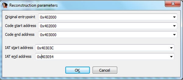
Now choose whichever method suits you best and find the correct address. In our case the original entry point address is 0x402000. This also happens to be the start of our source code so we can already supply two uunp input fields with the correct data (see Figure 11). The next field is ‘Code end address’ – if you can’t get it from the unpacking loop then treat that as your homework. For now you can cheat a bit and load the original, unpacked test file into IDA and get this data from the ‘Segments’ view option.
Next we need the IAT start and end addresses. Obviously, IAT requires the result of the GetProcAddress function. If you analyse the depacking loop closely you can see that GetProcAddress is being called at address .MPRESS1:0000000000401152. Insert a breakpoint on the instruction before the GetProcAddress call (.MPRESS1:000000000040114F mov rcx, rbx) and run the process. When the breakpoint is hit, note the RDI register value. This is our starting address. Run the code again and after the last call to GetProcAddress execute the stosq instruction:
.MPRESS1:000000000040114F loc_40114F:                  ; CODE XREF: .MPRESS1:0000000000401141j
.MPRESS1:000000000040114F mov     rcx, rbx             ; hModule
.MPRESS1:0000000000401152 call    GetProcAddress
.MPRESS1:0000000000401157 stosq
Now note the RDI register value. This will be the IAT end address we are looking for. Now you can place a breakpoint at the original entry point (at 0x040200) and resume process execution. When the breakpoint at the OEP is hit, invoke uunp from the ‘Edit->Plug-ins-> Universal Unpacker Manual Reconstruct’ option and enter the data as shown in Figure 11. This should result in a fixed IAT and a more readable disassembly of our unpacked code as shown in Figure 13; Figure 12 contains the original unpacked code prior to running uunp.
IDA has the option to be run with a temporary database instead of creating a normal database. This can be achieved with the -t option. A temporary database might be useful when unpacking a file with a debugger in several attempts, for example.
IDA has very limited undo functionality – this means that if you break something you might not be able to quickly return it to the previous state. This is why database snapshot functionality is so handy: use it during manual analysis and unpacking! On the other hand, temporary databases are a nice feature when you want the final database to be free from any middle stages and mistakes you’ve made during initial attempts.
The TakeMemorySnapshot() function is available from IDAPython, so according to the previous tips, use it!
Do not forget to apply FLIRT signatures to uncompressed/deobfuscated code areas as it can aid further analysis enormously. Let IDA do the dirty work.
When stopping debugger execution from script do not forget to call GetDebuggerEvent() before the next call.
Source code for uunp and the Universal PE Unpacker plug-in is available in the IDA SDK so you can peek into the internals of them both. This can be helpful when designing your own solution.
While unpacking and IAT rebuilding techniques do not differ much in general between PE and PE32+ files, the publicly available toolset is still lacking behind x64 files. Some 32-bit tools including scripts and plug-ins might not work against x64 compression/obfuscation utilities, however the background in unpacking 32-bit executables is more than helpful when unpacking 64-bit modules. The solutions and methods presented in this tutorial series aimed to show a broad spectrum of the problem and provide ready-to-use tools in order to enable solving of more complex issues by introducing solid foundations. Remember that mpress does not obfuscate code – it just compresses it – and it does not contain any anti-debugging/anti-disassembly tricks. This is an ideal situation that does not happen every time in the case of malware analysis. You can also count on the appearance of a new set of anti-debugging tricks for x64 platforms – but, by now, you should be well prepared to battle those.