2008-05-01
Abstract
Malware researchers are frequently faced with huge collections of files that must be analysed to determine whether or not they are malware. In such situations, grouping the files according to their binary similarity can save time and effort. Víctor Álvarez discusses the algorithms that can be used to make the life of the malware researcher easier.
Copyright © 2008 Virus Bulletin
Malware researchers often need to group large sets of files according to their binary similarity. For instance, they are frequently faced with huge collections of files that must be analysed to determine whether or not they are malware. Such collections generally contain files which are very similar, but which do not match exactly, while many other files bear no relation to the rest. In such a situation, grouping the files according to their binary similarity can save a lot of time and effort. In this article we will discuss some algorithms that can be used for this purpose.
The first thing we need to do before we can implement an algorithm for grouping similar files is to define a way to measure the grade of similarity between two given files. From now on, we will refer to this grade of similarity as the distance between the two files. The more similar the files, the smaller the distance between them and vice-versa.
A good way to measure the distance between two files is to calculate the length of their longest common subsequence.
Let A be a sequence of symbols of length m, then a subsequence of A is another sequence, A´, of length n ≤ m that can be obtained by removing zero or more symbols from A. For example, abce, bcde, bad, and ade are all subsequences of abacde. Obviously, the longest common subsequence (LCS) of A and B is the longest sub-sequence of A that is also a subsequence of B.
Although the length of the longest common subsequence (LLCS) is theoretically a good measure of file similarity, it has a major drawback in practice: its time complexity. Several algorithms for solving the LCS and LLCS problems have been proposed by different authors, including Hirschberg [1] Hunt and Szymanski [2], Kuo and Cross [3] and some others, but all of them run in quadratic time. Taking into account the large number of file comparisons needed to cluster a large set of files, it is obvious that a linear time algorithm for calculating file distances is preferred, even at the expense of losing accuracy in the measurement.
That’s when delta algorithms come into play. The purpose of delta algorithms is to receive two files and generate a set of instructions that can be used to convert one of the files into the other. In other words, given the reference file A and the target file B, a delta algorithm is composed of two functions Δg and Δp such that:
Δg (A,B) = C and Δp (A,C) = B
The function Δg generates a set of instructions C that can be used in conjunction with A to obtain B using Δp. This kind of algorithm is widely used for performing incremental data backups, distributing software updates, and many more situations where changes must be made to existing data and it is more efficient to send or store just the difference between versions than the whole new set of data.
Delta algorithms are strongly related to the LCS problem. The relationship becomes more evident when considering that the LCS and the string-to-string correction problem (STSC) are dual (i.e. the two problems are complementary, a solution to one of them determines a solution to the other).
The STSC problem consists of finding the minimum number of insertions and deletions necessary to convert a given sequence of symbols into another. In fact, some delta algorithms rely on solving the LCS/STSC problem to find the shortest possible delta file, but many of them don’t pretend to find the optimal set of instructions, they just try to find one that is good enough, sacrificing solution quality in favour of execution speed.
The algorithm we will present here to calculate the distance between two files is inspired by xdelta [4]. Both the reference file F1 and the target file F2 are scanned simultaneously with an offset of W bytes. The scanning of F2 starts when the first W bytes of F1 have been scanned (in our tests we set W to 64 KB with good results).
On each increment of the current position of F1 four bytes are read from the file, passed through a hash function H, and the result is used as an index on the hash table T where the current position of F1 is stored. The hash table does not chain hash collisions; when a collision occurs the previous value is overwritten.
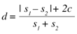
When scanning F2 four bytes are also read on each iteration. The hash table is used to find out if there is a match in F1 for these four bytes. If a match is found, the current position of F2 advances until the end of the matching block – this would generate a copy instruction in the output of the xdelta algorithm. If there is no match the current position of F2 is incremented. This would generate an insert instruction. The distance d between the two files is based on the number of instructions c that would be generated, and the size of both files s1 and s2, following the expression:
It must be said that this distance is not symmetrical (i.e. d(A,B) ≠ d(B,A) ), although it tends to be more symmetrical when the files are more similar. For files with very dissimilar sizes, but which are still similar in some way (consider, for example, the case of comparing a file with a truncated version of itself), this asymmetry could lead to very different results depending on the order of comparison. To avoid this discrepancy, we decided that the biggest file would always be the reference file F1, and the smallest one the target file F2. This is because the delta algorithm generates fewer instructions when trying to convert a large file into a smaller one than the opposite way round.
Here is the algorithm for calculating the number of instructions c in more detail:
(1) while F1 [i] = F2 [i] do i ← i + 1
(2) if (i = s2) return 0
(3) for i ≤ j < i + W do
      x ← four bytes of F1 at offset j
      T[H(x)] ← j
      j ← j + 1
(4) c ← c + 1
    x ← four bytes of F2 at offset i
    k ← T[H(x)]
    if (k is null)
      x ← four bytes of F1 at offset j
      T[H(x)] ← j
      j ← j + 1
      i ← i + 1
    else while (F1 [k] = F2 [i]) do
            x ← four bytes of F1 at offset j
            T[H(x)] ← j
            j ← j + 1
            i ← i + 1
            k ← k + 1
(5)  repeat (4) until end of F2
(6)  return c
Once we have defined a metric to measure file similarity, the next part of our problem is to find a method for grouping similar files together. This is when clustering algorithms become helpful. In general terms, clustering algorithms are aimed at partitioning a set of objects into subsets according to their proximity, as defined by some distance measure.
An incredible number of clustering algorithms have been developed over the years for different purposes and employing a variety of techniques. Terms like ‘K-means’, ‘fuzzy C-means’ and ‘hierarchical clustering’ populate hundreds of academic and research papers across a broad spectrum of fields, and there are plenty of choices for a clustering algorithm. However, the characteristics of the problem we wanted to solve meant that it was not difficult to choose an appropriate algorithm for our needs.
From the very beginning it was obvious that algorithms like K-means, which rely on finding a centroid for each cluster, were not suitable in this case. A centroid is nothing more than a central point for a cluster or group of objects, which is not necessarily one of the objects. Depending on the nature of the objects we want to cluster, establishing the centroid for a cluster could be an easy or a very difficult task. Calculating the centroid of n points in a Euclidean space is straightforward, but establishing a centroid for a group of files is a whole new problem on its own. K-medoids, another clustering algorithm very similar to K-means, does not have this problem because the central point for each cluster (or medoid) is not external to the objects, but one of the objects itself. However, both algorithms need to know in advance the number of clusters into which the data will be partitioned – a requirement that makes these algorithms unsuitable for our purposes.
On the other hand, hierarchical clustering algorithms seemed very appropriate for the task. There are different variants of hierarchical clustering algorithms, but we will concentrate on agglomerative single linkage clustering. This algorithm starts by placing each object (a file in our case) in a separate cluster. At each stage of the algorithm the two closest clusters are merged together until a certain number of clusters is reached, or until the distance between the two closest clusters exceeds a predefined value. The distance d between two clusters Cn and Cm is defined as the minimum distance between any object from Cn and any object from Cm.
In a more formal way:
d(Cn,Cm) = min { d(x,y) | x ∈ Cn, y ∈ Cm}
In order to see the algorithm in a more detailed way let’s assume that we have N files Fn (1 ≤ n ≤ N) to cluster, C denotes a cluster, and df is the minimum distance allowed between any two clusters of the final result, then:
Construct matrix D of dimensions N × N such that:
Dnm= d(Cn,Cm) = d(Fn,Fm) n ≤ N, m < n
(as d(Fn,Fm) = d(Fm,Fn), D is symmetrical and only the lower half is used)
Find clusters Cx and Cy such that:
d(Cx,Cy) = min { d(Cn,Cm) | n ≤ N, m < n }
Merge Cx and Cy into a single cluster Cx ∪ Cy and reconstruct D by removing the two rows and columns that correspond to Cx and Cy and adding a new row and a new column for the newly created Cx ∪ Cy. Now N ← N –1 and the distance from any existing cluster Cp to the new cluster Cx ∪ Cy is given by:
d(Cp, Cx ∪ Cy) = min { d(Cp,Cx), d(Cp,Cy) }
Repeat from step (2) while there is more than one cluster and the distance between the two closest clusters does not exceed df.
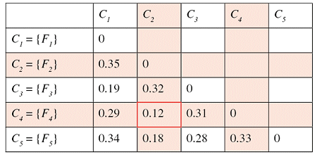
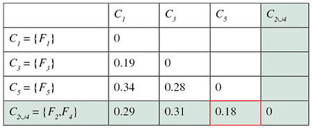
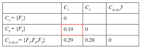
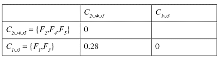
Successive steps of the algorithm applied to a set of five files are shown in the tables below. The minimum distance in the first matrix is between clusters C2 and C4. The corresponding columns and rows (in red) are deleted from the first matrix and a new row and column (in green) are added to construct the second. The algorithm continues until the distance between the two closest clusters is greater than df = 0.25.
The result of this clustering algorithm is a hierarchical representation of similarity between the files, which is usually called a dendrogram. In a dendrogram each leaf of the tree is an element of the set being clustered, and each node in the middle of the tree represents an association between two objects, one cluster and one object, or two clusters. The picture below, showing the dendrogram corresponding to our previous example with five files, speaks for itself.
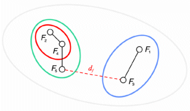
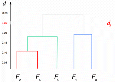
Notice that as the algorithm is interrupted when the distance between the two closest clusters is greater than df, a set of sub-trees is obtained instead of a single tree. All elements that are leaves of the same sub-tree are also members of the same cluster in the final result of the algorithm.
File clustering is a costly process. The number of file comparisons that must be done to fill the initial distance matrix for the clustering algorithm is N × (N – 1) / 2. As the number of files grows linearly, the number of comparisons grows quadratically. The file comparison algorithm is not very costly in itself, it only depends linearly on the size of the files being compared, but it requires the content of both files to be read completely, incurring a large number of I/O disk operations with the obvious performance degradation that such operations impose. For this reason it is necessary to avoid unwanted file comparisons as much as possible.
A good heuristic is to avoid comparing files whose size is quite different. As a rule of thumb it can be said that a pair of files with sizes s1 and s2 should be compared only if they satisfy:
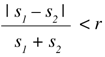
Here, r is a certain adjustable ratio that can be raised or lowered depending on the number of files, the characteristics of the hardware, and other factors. If the sizes do not satisfy the expression above, they are not compared and the distance between them is considered to be infinite.
Another possible optimization consists of aborting the distance computation when it is about to exceed a maximum value. As mentioned above, the clustering algorithm stops when the minimum distance between all existing clusters is greater than a given value we called df. Therefore, distances greater than df do not influence the final result - their values are irrelevant as long as they are greater than df. But the distance between two clusters is by definition the distance of their nearest elements, which means that it is also the distance between some pair of files in the set. When calculating such distances, the process can be interrupted at the very moment it exceeds df. This saves a considerable amount of file read operations, improving the general performance of the algorithm.
This article is based on well-known and studied algorithms; there is nothing genuinely new in what has been described here. However, I hope it may have served to show that mixing together existing algorithms and techniques in a creative way can sometimes help to improve the tools we have available to make our job easier.
I also hope this article may be relevant beyond the anti-virus industry, because grouping files according to their binary similarity has a broader range of applications than just sample categorization in malware analysis.
[1] Hirschberg, D.S. A linear space algorithm for computing maximal common subsequences. Communications of the ACM, volume 18, no. 6 (1975) pp.341–343.
[2] Hunt, J.; Szymanski, T.G. A fast algorithm for computing longest common subsequences. Communications of the ACM, volume 20, no. 5 (1977) pp.350–353.
[3] Kuo, S.; Cross, G.R. An improved algorithm to find the length of the longest common subsequence of two strings, ACM SIGIR Forum, volume 23, no. 3–4 (1989) pp.89–99.
[4] MacDonald, J.P. Versioned file archiving, compression, and distribution. University of California at Berkeley (1999). See http://citeseer.ist.psu.edu/macdonald99versioned.html.
[5] Burns, R.C.; Long, D.D.E. A linear time, constant space differencing algorithm. Proceedings of the International Performance, Computing and Communications Conference (IPCCC), IEEE, (1997).
[6] Hunt, J.J.; Vo, K-P.; Tichy, W.F. Delta algorithms: an empirical analysis. ACM Transactions on Software Engineering and Methodology, volume 7, no. 2 (1998) pp.192–214.